Working with JSON in ClickHouse

ClickHouse provides several approaches for handling JSON, each with its respective pros and cons and usage. In this guide, we will cover different approaches:

• Using type inference
• Using a structured approach
• Extraction of values at query time
• Using maps
• Using paired arrays

note

A new JSON type is being actively developed and will be available soon. You can track the progress of this feature by following this GitHub issue. This new data type will replace the existing deprecated JSON object.

Type Inference

When to use type inference:

• The data from which you are going to infer types contains all the columns that you are interested with. Data with additional columns added after the type inference will be ignored and can't be queried.
• Data types for a specific columns need to be compatible

If your data is structured and your data is in JSON format, you don't have to spend time defining your table DDL and selecting the types of each columns to match your data. ClickHouse can do it for you using type inference. Let's see how it can do it using the following dataset:

SELECT
    *
FROM s3('https://storage.googleapis.com/clickhouse_public_datasets/pypi/sample/*.json.gz', 'NOSIGN', 'JSONEachRow')
WHERE project = 'requests'
LIMIT 5;

This dataset is stored in a GCS bucket and contains multiple files in JSON format. You can see that the files above contain rows with nested JSON object. Instead of building the DDL manually and spending time defining the type for each of the columns, you can see how ClickHouse will infer the type of each columns:

DESCRIBE TABLE s3('https://storage.googleapis.com/clickhouse_public_datasets/pypi/sample/*.json.gz') FORMAT TSV;

This should return each column with their corresponding types:

timestamp   Nullable(DateTime64(9))                 
country_code    Nullable(String)                    
url Nullable(String)                    
project Nullable(String)                    
file    Tuple(filename Nullable(String), project Nullable(String), type Nullable(String), version Nullable(String))                 
details Tuple(cpu Nullable(String), distro Tuple(id Nullable(String), libc Tuple(lib Nullable(String), version Nullable(String)), name Nullable(String), version Nullable(String)), implementation Tuple(name Nullable(String), version Nullable(String)), installer Tuple(name Nullable(String), version Nullable(String)), openssl_version Nullable(String), python Nullable(String), rustc_version Nullable(String), setuptools_version Nullable(String), system Tuple(name Nullable(String), release Nullable(String)))                 
tls_protocol    Nullable(String)                    
tls_cipher  Nullable(String)    

You can see a lot of the columns are detected as Nullable. We do not recommend using the Nullable type when not absolutely needed. You can use schema_inference_make_columns_nullable to control the behavior of when Nullable is applied.

CREATE TABLE pypi
ENGINE = MergeTree
ORDER BY (project, timestamp) EMPTY AS
SELECT *
FROM s3('https://storage.googleapis.com/clickhouse_public_datasets/pypi/sample/*.json.gz') SETTINGS schema_inference_make_columns_nullable = 0;

In the query above we created a table based on the inference ClickHouse did on the data present in the GCS bucket.

SHOW CREATE TABLE pypi;

The query above will show you the table that was created with the corresponding type of each column. You can now insert the data into your table using the following query:

INSERT INTO pypi SELECT * FROM s3('https://storage.googleapis.com/clickhouse_public_datasets/pypi/sample/*.json.gz', 'NOSIGN', 'JSONEachRow')
WHERE project = 'requests';

Handling errors

Sometimes, you might have bad data, for example a specific columns that doesn't have the right type, or an improperly formatted JSON, you can use the setting input_format_allow_errors_ratio to allow a certain number of rows to be ignored if the data are triggering insert errors.

Further reading

To learn more about the data type inference you can refer to this documentation page.

Other Approaches

These approaches can be summarized as follows:

• Handle as structured data - explicitly map each column and ensure that the table schema is maintained if new data is added. We can exploit the tuple, map, and nested data types in this case for nested structures.
• Store as a string - using functions to extract properties at query time or potentially adding materialized columns as needed
• Utilize the map type - use the Map type to store homogenous key-value pair
• Utilize paired arrays - store the data as arrays of keys and values

We address each of these below and discuss their benefits and limitations.

For our example, we use a simple logging dataset, a sample of which is shown below. Although the full dataset contains over 200m rows, which the user is free to download, only a sample is used in most cases to ensure queries are responsive.

{
  "@timestamp": 893964617,
  "clientip": "40.135.0.0",
  "request": {
    "method": "GET",
    "path": "/images/hm_bg.jpg",
    "version": "HTTP/1.0"
  },
  "status": 200,
  "size": 24736
}

The full dataset is available in s3 as numbered files of the format documents-<01-25>.tar.gz. We utilize the first of these files documents-01.tar.gz to ensure sample queries execute promptly:

SELECT * FROM s3('https://datasets-documentation.s3.eu-west-3.amazonaws.com/http/documents-01.ndjson.gz',
'JSONEachRow') LIMIT 1;

@timestamp	clientip	request	status	size
893964617	40.135.0.0	{'method':'GET','path':'/images/hm_bg.jpg','version':'HTTP/1.0'}	200	24736

Handle as Structured Data

If your JSON has a fixed schema, mapping it to an explicit schema provides the most optimal performance. Specifically, users can control codecs, configure data skipping indexes and utilize columns in primary and sort keys.

This approach represents the most optimal means of handling JSON. It is limited in a number of ways, however, specifically:

• JSON values need to be consistent and mappable to columns. If the data is inconsistent or dirty, insert logic will need to be modified.
• All columns and their types must be known upfront. Changes will need to be made to the table should JSON keys be added - prior knowledge of this is required.

For the example above, most of the fields have obvious types. However, we have a few options for the object request field: nested, tuple, and map (assuming no support for JSON objects).

Using Nested

Below we provide an example of using nested.

CREATE table http
(
   `@timestamp` Int32 EPHEMERAL 0,
   clientip     IPv4,
   request Nested(method LowCardinality(String), path String, version LowCardinality(String)),
   status       UInt16,
   size         UInt32,
   timestamp    DateTime DEFAULT toDateTime(`@timestamp`)
) ENGINE = MergeTree() ORDER BY (status, timestamp);

SET input_format_import_nested_json = 1;
INSERT INTO http (`@timestamp`, clientip, request.method, request.path, request.version, status, size)
FORMAT JSONEachRow
   {"@timestamp":897819077,"clientip":"45.212.12.0","request":{"method":["GET"],
   "path":["/french/images/hm_nav_bar.gif"],"version":["HTTP/1.0"]},"status":200,"size":3305}

A few important points to note here:

• We need to use the setting input_format_import_nested_json to insert the JSON as a nested structure. Without this, we are required to flatten the JSON i.e.

  INSERT INTO http_uint FORMAT JSONEachRow
  {"@timestamp":897819077,"clientip":"45.212.12.0","request.method":["GET"],
  "request.path":["/french/images/hm_nav_bar.gif"],"request.version":["HTTP/1.0"],
  "status":200,"size":3305}

• The nested fields method, path, and version need to be passed as JSON arrays

• The columns must be specified in INSERT - this is actually because of the EPHEMERAL column @timestamp, which requires a type conversion.

Columns can be queried using a dot notation.

SELECT clientip, status, size, `request.method` FROM http WHERE has(request.method, 'GET');

Notice how we are required to query request.method as an Array. It is easiest to think of a nested data structure as multiple column arrays of the same length. The fields method, path, and version are all separate Array(Type) columns in effect with one critical constraint: the length of the method, path, and version fields must be the same.

If your nested structure fits this constraint, and you are comfortable ensuring the values are inserted as strings, nested provides a simple means of querying JSON. Note the use of Arrays for the sub-columns means the full breath Array functions can potentially be exploited, including the Array Join clause - useful if your columns have multiple values. Additionally, nested fields can be used in primary and sort keys.

Given the constraints and input format for the JSON, we insert our sample dataset using the following query. Note the use of the map operators to access the request fields - this results from schema inference detecting a map for the request field in the s3 data.

The following statement inserts 10m rows, so this may take a few minutes to execute. Apply a LIMIT if required.

INSERT INTO http (`@timestamp`, clientip, request.method, request.path, request.version, status, size)
SELECT `@timestamp`, clientip, [request['method']], [request['path']], [request['version']], status,
size FROM s3('https://datasets-documentation.s3.eu-west-3.amazonaws.com/http/documents-01.ndjson.gz',
'JSONEachRow');

Querying this data requires us to access the request fields as arrays. Below we summarize the errors and http methods over a fixed time period.

SELECT status, request.method[1] as method, count() as c
FROM http
WHERE status >= 400
  AND timestamp BETWEEN '1998-01-01 00:00:00' AND '1998-06-01 00:00:00'
GROUP by method, status
ORDER BY c DESC LIMIT 5;

status	method	c
404	GET	11267
404	HEAD	276
500	GET	160
500	POST	115
400	GET	81

Using Tuples

The nested object request can also be represented as a Tuple. This provides comparable functionality to nested, addressing some of its constraints at the expense of other limitations. For example, by not using Arrays we do not have the same constraint that subfields of an object have to be the same length. This lets us represent more varied structures. However, unlike nested fields, the subfields of tuples cannot be used in primary and sort keys.

First, create an example table for the http data:

DROP TABLE IF EXISTS http;

CREATE table http
(
    `@timestamp` Int32 EPHEMERAL 0,
    clientip     IPv4,
    request Tuple(method LowCardinality(String), path String, version LowCardinality(String)),
    status       UInt16,
    size         UInt32,
    timestamp    DateTime DEFAULT toDateTime(`@timestamp`)
) ENGINE = MergeTree() ORDER BY (status, timestamp);

Insertion of data requires changes to the nested field structure. Specifically, note how the “request” object below must be passed as an array of values.

INSERT INTO http (`@timestamp`, clientip, request, status, size) FORMAT JSONEachRow
    {"@timestamp":893964617,"clientip":"40.135.0.0","request":["GET", "/images/hm_bg.jpg", "HTTP/1.0"],
    "status":200,"size":24736}

We have minimal data in our example above, but as shown below we can query the tuple fields by their period delimited names. We also aren’t required to use Array functions like nested.

SELECT `request.method`, status, timestamp FROM http WHERE request.method = 'GET';

request.method	status	timestamp
GET	200	1998-04-30 19:30:17

The principal disadvantage of tuples, other than the requirement to convert our objects into lists, is the sub fields cannot be used as primary or sort keys. The following will thus fail.

DROP TABLE IF EXISTS http;

CREATE table http
(
   `@timestamp` Int32 EPHEMERAL 0,
   clientip     IPv4,
   request Tuple(method LowCardinality(String), path String, version LowCardinality(String)),
   status       UInt16,
   size         UInt32,
   timestamp    DateTime DEFAULT toDateTime(`@timestamp`)
) ENGINE = MergeTree() ORDER BY (status, request.method, timestamp);

However, the entire tuple can be used for this purpose. The following is valid.

DROP TABLE IF EXISTS http;

CREATE table http
(
   `@timestamp` Int32 EPHEMERAL 0,
   clientip     IPv4,
   request Tuple(method LowCardinality(String), path String, version LowCardinality(String)),
   status       UInt16,
   size         UInt32,
   timestamp    DateTime DEFAULT toDateTime(`@timestamp`)
) ENGINE = MergeTree() ORDER BY (status, request, timestamp);

To insert our sample data from s3 we can use the following query. Note the need to form a tuple at insert time for the request field i.e. (request['method'], request['path'], request['version']).

INSERT INTO http(`@timestamp`, clientip, request, status, size) SELECT `@timestamp`, clientip,
(request['method'], request['path'], request['version']), status, size FROM
s3('https://datasets-documentation.s3.eu-west-3.amazonaws.com/http/documents-01.ndjson.gz',
'JSONEachRow');

To reproduce our earlier query analyzing error rates by status code, we don’t require any special syntax:

SELECT status, request.method as method, count() as c
FROM http
WHERE status >= 400
  AND timestamp BETWEEN '1998-01-01 00:00:00' AND '1998-06-01 00:00:00'
GROUP by method, status
ORDER BY c DESC LIMIT 5;

Using Maps

Maps represent a simple way to represent nested structures, with some noticeable limitations:

• The fields must be of all the same type.
• Accessing subfields requires a special map syntax - since the fields don’t exist as columns i.e. the entire object is a column.

Provided we assume the subfields of our request object are all Strings, we use a map to hold this structure.

DROP TABLE IF EXISTS http;
CREATE table http
(
   `@timestamp` Int32 EPHEMERAL 0,
   clientip     IPv4,
   request Map(String, String),
   status       UInt16,
   size         UInt32,
   timestamp    DateTime DEFAULT toDateTime(`@timestamp`)
) ENGINE = MergeTree() ORDER BY (status, request, timestamp);

Unlike Nested and Tuple, we aren’t required to make changes to our JSON structures at insertion.

INSERT INTO http (`@timestamp`, clientip, request, status, size) FORMAT JSONEachRow
    {"@timestamp":897819077,"clientip":"45.212.12.0","request":{"method": "GET","path":"/french/images/hm_nav_bar.gif","version":"HTTP/1.1"},"status":200,"size":3305}

Querying these fields within the request object requires a map syntax e.g.

SELECT * FROM http;

clientip	request	status	size	timestamp
45.212.12.0	{'method':'GET','path':'/french/images/hm_nav_bar.gif','version':'HTTP/1.1'}	200	3305	1998-06-14 10:11:17

SELECT timestamp, request['method'] as method, status FROM http WHERE request['method'] = 'GET';

timestamp	method	status
1998-06-14 10:11:17	GET	200

A full set of map functions is available to query this time, described here. If your data is not of a consistent type, functions exist to perform the necessary coercion. The following example, exploits the fact that data objects can also be inserted into a map in the structure [(key, value), (key, value),...] e.g. [('method', 'GET'),('path', '/french/images/hm\_nav\_bar.gif'),('version', 'HTTP/1.1')]

This function in turn allows us to insert our full s3 dataset with no need to reformat the data.

INSERT INTO http (`@timestamp`, clientip, request,
status, size) SELECT `@timestamp`, clientip, request, status, size FROM
s3('https://datasets-documentation.s3.eu-west-3.amazonaws.com/http/documents-01.ndjson.gz',
'JSONEachRow');

To reproduce our earlier query example which analyzes status codes by HTTP method, we require the use of the map syntax:

SELECT status, request['method'] as method, count() as c
FROM http
WHERE status >= 400
 AND timestamp BETWEEN '1998-01-01 00:00:00' AND '1998-06-01 00:00:00'
GROUP by method, status
ORDER BY c DESC LIMIT 5;

Nested vs Tuple vs Map

Each of the above strategies for handling nested JSON has its respective advantages and disadvantages. The following captures these differences.

Type	Requires custom INSERT format	Requires custom notation to read fields	Constraints on structure e.g. list lengths or types	Object fields can be used for primary/sort keys	Creates more columns on disk
Nested	Yes	No	Yes*	Yes	Yes
Tuple	Yes	No	No	No	No
Map	No	Yes	Yes**	No	No

*Nested requires values (represented as arrays) to have the same length **Values must be the same type

Store as String

Handling data using the structured approach described in Handle as Structured Data, is often not viable for those users with dynamic JSON which is either subject to change or for which the schema is not well understood. For absolute flexibility, users can simply store JSON as Strings before using functions to extract fields as required. This represents the extreme opposite to handling JSON as a structured object. This flexibility incurs costs with significant disadvantages - primarily an increase in query syntax complexity as well as degraded performance.

Our table schema, in this case, is trivial:

DROP TABLE IF EXISTS http;
CREATE table http_json
(
   message String

) ENGINE = MergeTree ORDER BY tuple();

Insertion requires us to send each JSON row as a String. Here we use the format JSONAsString to ensure our object is interpreted.

INSERT INTO http FORMAT JSONAsString
  {"@timestamp":897819077,"clientip":"45.212.12.0","request":{"method":"GET",
  "path":"/french/images/hm_nav_bar.gif","version":"HTTP/1.0"},"status":200,"size":3305}

To illustrate queries we can insert our sample from s3:

INSERT INTO http SELECT * FROM s3('https://datasets-documentation.s3.eu-west-3.amazonaws.com/http/documents-01.ndjson.gz',
'JSONAsString');

The below query counts the requests with a status code greater than 200, grouping by HTTP method.

SELECT JSONExtractString(JSONExtractString(message, 'request'), 'method') as method,
       JSONExtractInt(message, 'status')                                  as status,
       count()                                                            as count
FROM http
WHERE status >= 400
  AND method == 'GET'
GROUP BY method, status;

method	status	count
GET	404	11267
GET	400	81
GET	500	160

Despite using functions to parse the String, this query should still return for the 10m rows in a few seconds. Notice how the functions require both a reference to the String field message and a path in the JSON to extract. Nested paths require functions to be nested e.g. JSONExtractString(JSONExtractString(message, 'request'), 'method') extracts the field request.method. The extraction of nested paths can be simplified through the functions JSON_QUERY AND JSON_VALUE as shown below:

SELECT JSONExtractInt(message, 'status') AS status, JSON_VALUE(message, '$.request.method') as method,
count() as c
FROM http
WHERE status >= 400
  AND toDateTime(JSONExtractUInt(message, '@timestamp')) BETWEEN '1998-01-01 00:00:00'
  AND '1998-06-01 00:00:00'
GROUP by method, status
ORDER BY c DESC LIMIT 5;

status	method	c
404	GET	11267
404	HEAD	276
500	GET	160
500	POST	115
400	GET	81

Notice the use of an xpath expression here to filter the JSON by method i.e. JSON_VALUE(message, '$.request.method').

String functions are appreciably slower (> 10x) than explicit type conversions with indices. The above queries always require a full table scan and processing of every row. While these queries will still be fast on a small dataset such as this, performance will degrade on larger datasets.

The flexibility this approach provides comes at a clear performance and syntax cost. It can, however, be coupled with other approaches where users extract only the explicit fields they need for indices or frequent queries. For further details on this approach, see Hybrid approach.

Visit Functions

The above examples use the JSON* family of functions. These utilize a full JSON parser based on simdjson, that is rigorous in its parsing and will distinguish between the same field nested at different levels. These functions are able to deal with JSON that is syntactically correct but not well-formatted, e.g. double spaces between keys.

A faster and more strict set of functions are available. These visitParam* functions offer potentially superior performance, primarily by making strict assumptions as to the structure and format of the JSON. Specifically:

• Field names must be constants

• Consistent encoding of field names e.g. visitParamHas('{"abc":"def"}', 'abc') = 1, but visitParamHas('{"\u0061\u0062\u0063":"def"}', 'abc') = 0

• The field names are unique across all nested structures. No differentiation is made between nesting levels, and matching is indiscriminate. In the event of multiple matching fields, the first occurrence is used.

• No special characters outside of string literals. This includes spaces. The following is invalid and will not parse.

  {"@timestamp": 893964617, "clientip": "40.135.0.0", "request": {"method": "GET",
  "path": "/images/hm_bg.jpg", "version": "HTTP/1.0"}, "status": 200, "size": 24736}

  whereas, will parse correctly

  {"@timestamp":893964617,"clientip":"40.135.0.0","request":{"method":"GET",
  "path":"/images/hm_bg.jpg","version":"HTTP/1.0"},"status":200,"size":24736}

In some circumstances, where performance is critical and your JSON meets the above requirements, these may be appropriate. An example of the earlier query, re-written to use visitParam functions is shown below:

SELECT visitParamExtractUInt(message, 'status')   AS status,
       visitParamExtractString(message, 'method') as method,
       count()                                    as c
FROM http
WHERE status >= 400
  AND toDateTime(visitParamExtractUInt(message, '@timestamp')) BETWEEN '1998-01-01 00:00:00' AND '1998-06-01 00:00:00'
GROUP by method, status
ORDER BY c DESC LIMIT 5;

status	method	c
404	GET	11267
404	HEAD	276
500	GET	160
500	POST	115
400	GET	81

Note that these functions are also aliased to simpleJSON* equivalents. The above query can be rewritten to:

SELECT simpleJSONExtractUInt(message, 'status')   AS status,
       simpleJSONExtractString(message, 'method') as method,
       count()                                    as c
FROM http
WHERE status >= 400
  AND toDateTime(simpleJSONExtractUInt(message, '@timestamp')) BETWEEN '1998-01-01 00:00:00'
  AND '1998-06-01 00:00:00'
GROUP by method, status;

Using Pairwise Arrays

Pairwise arrays provide a balance between the flexibility of representing JSON as Strings and the performance of a more structured approach. The schema is flexible in that any new fields can be potentially added to the root. This, however, requires a significantly more complex query syntax and isn’t compatible with nested structures.

As an example, consider the following table:

CREATE TABLE http_with_arrays (
   keys Array(String),
   values Array(String)
)
ENGINE = MergeTree  ORDER BY tuple();

To insert into this table, we need to structure the JSON as a list of keys and values. The following query illustrates the use of the JSONExtractKeysAndValues to achieve this:

SELECT arrayMap(x -> x.1, JSONExtractKeysAndValues(json, 'String')) as keys,
       arrayMap(x -> x.2, JSONExtractKeysAndValues(json, 'String')) as values
FROM s3('https://datasets-documentation.s3.eu-west-3.amazonaws.com/http/documents-01.ndjson.gz',
'JSONAsString') LIMIT 1;

keys	values
['@timestamp','clientip','request','status','size']	['893964617','40.135.0.0','{"method":"GET","path":"/images/hm_bg.jpg","version":"HTTP/1.0"}','200','24736']

Note how the request column remains a nested structure represented as a string. We can insert any new keys to the root. We can also have arbitrary differences in the JSON itself. To insert into our local table, execute the following:

INSERT INTO http_with_arrays
SELECT arrayMap(x ->
                    x.1, JSONExtractKeysAndValues(message, 'String')) keys
FROM s3('https://datasets-documentation.s3.eu-west-3.amazonaws.com/http/documents-01.ndjson.gz',
'JSONEachRow');

Querying this structure requires using the indexOf function to identify the index of the required key (which should be consistent with the order of the values). This can in turn be used to access the values array column i.e. values[indexOf(keys, 'status')]. We still require a JSON parsing method for the request column - in this case, simpleJSONExtractString.

SELECT toUInt16(values[indexOf(keys, 'status')])                           as status,
       simpleJSONExtractString(values[indexOf(keys, 'request')], 'method') as method,
       count()                                                             as c
FROM http_with_arrays
WHERE status >= 400
  AND toDateTime(values[indexOf(keys, '@timestamp')]) BETWEEN '1998-01-01 00:00:00' AND '1998-06-01 00:00:00'
GROUP by method, status ORDER BY c DESC LIMIT 5;

status	method	c
404	GET	11267
404	HEAD	276
500	GET	160
500	POST	115
400	GET	81

Hybrid Approach with Materialized Columns

The approaches outlined above are not either OR. While parsing JSON fields to structured columns offers the best query performance, it also potentially incurs the highest insertion overhead if done in ClickHouse. Practically, it is also sometimes not possible due to dirty or variable data or even potentially an unknown schema. Conversely, keeping the JSON as Strings or using pairwise arrays, while flexible, significantly increases query complexity and makes accessing the data the function of someone with ClickHouse expertise.

As a compromise, users can use a hybrid approach: representing the JSON as a String initially, extracting columns as required. While not essential, Materialized Columns can assist with this.

For example, maybe we start with the following initial schema:

DROP TABLE IF EXISTS http;

CREATE table http
(
    message   String,
    method String DEFAULT JSONExtractString(JSONExtractString(message, 'request'), 'method'),
    status    UInt16 DEFAULT toUInt16(JSONExtractInt(message, 'status')),
    size      UInt32 DEFAULT toUInt32(JSONExtractInt(message, 'size')),
    timestamp DateTime DEFAULT toDateTime(JSONExtractUInt(message, '@timestamp'))
) ENGINE = MergeTree() ORDER BY (status, timestamp);

Here we have simply moved our functions to extract data from the SELECT to DEFAULT values. This is somewhat of an artificial case as our JSON is simple and could, in reality, easily be mapped. Typically the columns extracted would be a small subset of a much larger schema.

INSERT INTO http (message) SELECT json as message
FROM s3('https://datasets-documentation.s3.eu-west-3.amazonaws.com/http/documents-01.ndjson.gz',
'JSONAsString');

At this point, we may decide we need to add the column client_ip after querying it frequently:

ALTER TABLE http ADD COLUMN client_ip IPv4 DEFAULT toIPv4(JSONExtractString(message, 'clientip'));

The above change will only be incremental, i.e., the column will not exist for data inserted prior to the change. You can still query this column as it will be computed at SELECT time - although at an additional cost. Merges will also cause this column to be added to newly formed parts. To address this, we can use a mutation to update the existing data:

ALTER TABLE http UPDATE client_ip = client_ip WHERE 1 = 1

The second call here returns immediately and executes asynchronously. Users can track the progress of the update, which requires rewriting the data on disk, using the system.mutations table. Further details here. Note that this is a potentially expensive operation and should be scheduled accordingly. It is, however, more optimal than an OPTIMIZE TABLE <table_name> FINAL since it only writes the changed column.

Default vs Materialized

The use of default columns represents one of the ways to achieve “Materialized columns”. There is also a MATERIALIZED column syntax. This differs from DEFAULT in a few ways:

• MATERIALIZED columns cannot be provided on INSERT i.e. they must always be computed from other columns. Conversely, DEFAULT columns can be optionally provided.
• SELECT * will skip MATERIALIZED columns i.e. they must be specifically requested. This allows a table dump to be reloaded back into a table of the same definition.

Assessing Storage Usage

While extracting columns incurs a storage cost, typically, this can be minimized with a careful selection of codecs. Users will often wish to assess the cost of materializing a column prior. This cost only has a storage overhead if not queried - during the column-oriented nature of ClickHouse. We recommend testing the materialization on a subset of the data using a test table. The cost can, in turn, be computed using the following query, which can also provide an estimate of the compression achieved.

SELECT table,
      name,
      type,
      compression_codec,
      formatReadableSize(data_compressed_bytes)       as compressed_size,
      formatReadableSize(data_uncompressed_bytes)     as uncompressed_size,
      data_compressed_bytes / data_uncompressed_bytes as compression_ratio
FROM system.columns
WHERE database = currentDatabase()
ORDER BY table, name;

table	name	type	compression_codec	compressed_size	uncompressed_size	compression_ratio
http	client_ip	IPv4		23.51 MiB	38.15 MiB	0.61624925
http	message	String		203.00 MiB	1.48 GiB	0.1336674472634663
http	method	String		363.75 KiB	38.18 MiB	0.009304780749750751
http	size	UInt32		24.19 MiB	38.15 MiB	0.6341134
http	status	UInt16		87.49 KiB	19.07 MiB	0.00447955
http	timestamp	DateTime		4.98 MiB	38.15 MiB	0.1306381

Using Materialized Views

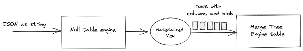
Using the hybrid approach described above requires significant processing at insertion time. This complicates data insertion logic and potentially introduces fragility in your data ingestion layer. To address this, we can exploit materialized views.

The general concept here is to exploit a table with the null engine for receiving inserts. This table engine doesn’t store any data and acts as a “buffer” for the materialized view only. For each insert block, the materialized view will trigger, perform the processing the required and insert rows into a target table that we can in turn query. In cases where we need to update the schema, extracting a new field from the blob, we simply update our table schema and then modify the materialized view accordingly to extract the field. Our materialized view and null table engine effectively act as an ETL pipeline, as shown below:

First, we create our null table engine for receiving inserts:

CREATE TABLE http_etl (
   message String
) ENGINE = Null;

Our target MergeTree table has a subset of the fields - ones we are maybe confident will occur in the JSON string. Note that we retain a String field message for other data that can be used with JSON* functions if required.

DROP TABLE IF EXISTS http;

CREATE table http
(
    message   String,
    method String,
    status    UInt16,
    size      UInt32,
    timestamp DateTime
) ENGINE = MergeTree() ORDER BY (status, timestamp);

Our materialized view in turn extracts the fields that have been declared in the http table schema.

CREATE MATERIALIZED VIEW http_mv TO http AS
SELECT message,
       JSONExtractString(JSONExtractString(message, 'request'), 'method') as method,
       toUInt16(JSONExtractInt(message, 'status'))                  as status,
       toUInt32(JSONExtractInt(message, 'size'))                       as size,
       toDateTime(JSONExtractUInt(message, '@timestamp')) as timestamp
FROM http_etl;

Using the sample data from our s3 bucket, the insert is simplified to:

INSERT INTO http_etl SELECT json as message FROM s3('https://datasets-documentation.s3.eu-west-3.amazonaws.com/http/documents-01.ndjson.gz',
'JSONAsString');

Our analysis of error codes and http methods thus becomes trivial:

SELECT status,
      method,
      count() as c
FROM http
WHERE status >= 400
 AND timestamp BETWEEN '1998-01-01 00:00:00' AND '1998-06-01 00:00:00'
GROUP by method, status ORDER BY c DESC;

Updating Materialized Views

Suppose we later wish to extract the field client_ip from our JSON blob. First we update our target table.

ALTER TABLE http
    ADD COLUMN client_ip IPv4;

Materialized view can be altered:

ALTER TABLE http_mv
   MODIFY QUERY SELECT message,
   JSONExtractString(JSONExtractString(message, 'request'), 'method') as method,
   toUInt16(JSONExtractInt(message, 'status')) as status,
   toUInt32(JSONExtractInt(message, 'size')) as size,
   toIPv4(JSONExtractString(message, 'clientip')) as client_ip,
   toDateTime(JSONExtractUInt(message, '@timestamp')) as timestamp
   FROM http_etl;

You can alternatively drop the view using DROP VIEW and recreate it - however this does require pausing insertions.

If an update of the target table is required, see the use of mutations in Hybrid Approach.

Using for Pairwise Arrays

In the above example, we represented fields we wished to frequently query explicitly as columns. A materialized view could also be potentially used to extract pairwise arrays. This shifts potentially expensive logic from the SELECT statement. For example:

CREATE TABLE http_with_arrays
(
   keys Array(String),
   values Array(String)
)
   ENGINE = MergeTree ORDER BY tuple();

CREATE MATERIALIZED VIEW http_mv TO http_with_arrays AS
SELECT arrayMap(x -> x.1, JSONExtractKeysAndValues(message, 'String')) as keys,
      arrayMap(x -> x.2, JSONExtractKeysAndValues(message, 'String')) as values
FROM http_etl;

INSERT INTO http_etl
SELECT json as message
FROM s3('https://datasets-documentation.s3.eu-west-3.amazonaws.com/http/documents-01.ndjson.gz',
'JSONAsString');

Importing JSON data

To import JSON data, we first have to define which JSON type to use. This will depend on how the input data is structured.

JSON tutorial

For a step by step tutorial with a large JSON dataset, please see Loading JSON in 5 steps.

Importing from an array of JSON objects

One of the most popular forms of JSON data is having a list of JSON objects in a JSON array, like in this example:

> cat list.json
[
  {
    "path": "Akiba_Hebrew_Academy",
    "month": "2017-08-01",
    "hits": 241
  },
  {
    "path": "Aegithina_tiphia",
    "month": "2018-02-01",
    "hits": 34
  },
  ...
]

Let’s create a table for this kind of data:

CREATE TABLE sometable
(
    `path` String,
    `month` Date,
    `hits` UInt32
)
ENGINE = MergeTree
ORDER BY tuple(month, path)

To import a list of JSON objects, we can use a JSONEachRow format (inserting data from list.json file):

INSERT INTO sometable
FROM INFILE 'list.json'
FORMAT JSONEachRow

We have used a FROM INFILE clause to load data from the local file, and we can see import was successful:

SELECT *
FROM sometable

┌─path──────────────────────┬──────month─┬─hits─┐
│ 1971-72_Utah_Stars_season │ 2016-10-01 │    1 │
│ Akiba_Hebrew_Academy      │ 2017-08-01 │  241 │
│ Aegithina_tiphia          │ 2018-02-01 │   34 │
└───────────────────────────┴────────────┴──────┘

Handling NDJSON (line delimited JSON)

Many apps can log data in JSON format so that each log line is an individual JSON object, like in this file:

cat object-per-line.json

{"path":"1-krona","month":"2017-01-01","hits":4}
{"path":"Ahmadabad-e_Kalij-e_Sofla","month":"2017-01-01","hits":3}
{"path":"Bob_Dolman","month":"2016-11-01","hits":245}

The same JSONEachRow format is capable of working with such files:

INSERT INTO sometable FROM INFILE 'object-per-line.json' FORMAT JSONEachRow;
SELECT * FROM sometable;

┌─path──────────────────────┬──────month─┬─hits─┐
│ Bob_Dolman                │ 2016-11-01 │  245 │
│ 1-krona                   │ 2017-01-01 │    4 │
│ Ahmadabad-e_Kalij-e_Sofla │ 2017-01-01 │    3 │
└───────────────────────────┴────────────┴──────┘

Importing from JSON object keys

In some cases, the list of JSON objects can be encoded as object properties instead of array elements (see objects.json for example):

cat objects.json

{
  "a": {
    "path":"April_25,_2017",
    "month":"2018-01-01",
    "hits":2
  },
  "b": {
    "path":"Akahori_Station",
    "month":"2016-06-01",
    "hits":11
  },
  ...
}

ClickHouse can load data from this kind of data using JSONObjectEachRow format:

INSERT INTO sometable FROM INFILE 'objects.json' FORMAT JSONObjectEachRow;
SELECT * FROM sometable;

┌─path────────────┬──────month─┬─hits─┐
│ Abducens_palsy  │ 2016-05-01 │   28 │
│ Akahori_Station │ 2016-06-01 │   11 │
│ April_25,_2017  │ 2018-01-01 │    2 │
└─────────────────┴────────────┴──────┘

Importing parent object key values

Let’s say we also want to save values in parent object keys to the table. In this case, we can use the following option to define the name of the column we want key values to be saved to:

SET format_json_object_each_row_column_for_object_name = 'id'

Now we can check which data is going to be loaded from the original JSON file using file() function:

SELECT * FROM file('objects.json', JSONObjectEachRow)

┌─id─┬─path────────────┬──────month─┬─hits─┐
│ a  │ April_25,_2017  │ 2018-01-01 │    2 │
│ b  │ Akahori_Station │ 2016-06-01 │   11 │
│ c  │ Abducens_palsy  │ 2016-05-01 │   28 │
└────┴─────────────────┴────────────┴──────┘

Note how the id column has been populated by key values correctly.

Importing from JSON arrays

Sometimes, for the sake of saving space, JSON files are encoded in arrays instead of objects. In this case, we deal with a list of JSON arrays:

cat arrays.json

["Akiba_Hebrew_Academy", "2017-08-01", 241],
["Aegithina_tiphia", "2018-02-01", 34],
["1971-72_Utah_Stars_season", "2016-10-01", 1]

In this case, ClickHouse will load this data and attribute each value to the corresponding column based on its order in the array. We use JSONCompactEachRow format for this:

SELECT * FROM sometable

┌─path──────────────────────┬──────month─┬─hits─┐
│ 1971-72_Utah_Stars_season │ 2016-10-01 │    1 │
│ Akiba_Hebrew_Academy      │ 2017-08-01 │  241 │
│ Aegithina_tiphia          │ 2018-02-01 │   34 │
└───────────────────────────┴────────────┴──────┘

Importing individual columns from JSON arrays

In some cases, data can be encoded column-wise instead of row-wise. In this case, a parent JSON object contains columns with values. Take a look at the following file:

cat columns.json

{
  "path": ["2007_Copa_America", "Car_dealerships_in_the_USA", "Dihydromyricetin_reductase"],
  "month": ["2016-07-01", "2015-07-01", "2015-07-01"],
  "hits": [178, 11, 1]
}

ClickHouse uses JSONColumns format to parse data formatted like that:

SELECT * FROM file('columns.json', JSONColumns)

┌─path───────────────────────┬──────month─┬─hits─┐
│ 2007_Copa_America          │ 2016-07-01 │  178 │
│ Car_dealerships_in_the_USA │ 2015-07-01 │   11 │
│ Dihydromyricetin_reductase │ 2015-07-01 │    1 │
└────────────────────────────┴────────────┴──────┘

A more compact format is also supported when dealing with an array of columns instead of an object using JSONCompactColumns format:

SELECT * FROM file('columns-array.json', JSONCompactColumns)

┌─c1──────────────┬─────────c2─┬─c3─┐
│ Heidenrod       │ 2017-01-01 │ 10 │
│ Arthur_Henrique │ 2016-11-01 │ 12 │
│ Alan_Ebnother   │ 2015-11-01 │ 66 │
└─────────────────┴────────────┴────┘

Saving JSON objects instead of parsing

There are cases you might want to save JSON objects to a single String (or JSON) column instead of parsing it. This can be useful when dealing with a list of JSON objects of different structures. Let's take this file where we have multiple different JSON objects inside a parent list:

cat custom.json

[
  {"name": "Joe", "age": 99, "type": "person"},
  {"url": "/my.post.MD", "hits": 1263, "type": "post"},
  {"message": "Warning on disk usage", "type": "log"}
]

We want to save original JSON objects into the following table:

CREATE TABLE events
(
    `data` String
)
ENGINE = MergeTree
ORDER BY ()

Now we can load data from the file into this table using JSONAsString format to keep JSON objects instead of parsing them:

INSERT INTO events (data)
FROM INFILE 'custom.json'
FORMAT JSONAsString

And we can use JSON functions to query saved objects:

SELECT
    JSONExtractString(data, 'type') AS type,
    data
FROM events

┌─type───┬─data─────────────────────────────────────────────────┐
│ person │ {"name": "Joe", "age": 99, "type": "person"}         │
│ post   │ {"url": "/my.post.MD", "hits": 1263, "type": "post"} │
│ log    │ {"message": "Warning on disk usage", "type": "log"}  │
└────────┴──────────────────────────────────────────────────────┘

Consider using JSONAsObject together with a new JSON data type to store and process JSON in tables in a more efficient way. Note that JSONAsString works perfectly fine in cases we have JSON object-per-line formatted files (usually used with JSONEachRow format).

Data types detection when importing JSON data

ClickHouse does some magic to guess the best types while importing JSON data. We can use a DESCRIBE clause to check which types were defined:

DESCRIBE TABLE file('list.json', JSONEachRow)

┌─name──┬─type─────────────┬─default_type─┬─default_expression─┬─comment─┬─codec_expression─┬─ttl_expression─┐
│ path  │ Nullable(String) │              │                    │         │                  │                │
│ month │ Nullable(Date)   │              │                    │         │                  │                │
│ hits  │ Nullable(Int64)  │              │                    │         │                  │                │
└───────┴──────────────────┴──────────────┴────────────────────┴─────────┴──────────────────┴────────────────┘

This allows quickly creating tables from JSON files:

CREATE TABLE new_table
ENGINE = MergeTree
ORDER BY tuple() AS
SELECT *
FROM file('list.json', JSONEachRow)

Detected types will be used for this table:

DESCRIBE TABLE new_table

┌─name──┬─type─────────────┬─default_type─┬─default_expression─┬─comment─┬─codec_expression─┬─ttl_expression─┐
│ path  │ Nullable(String) │              │                    │         │                  │                │
│ month │ Nullable(Date)   │              │                    │         │                  │                │
│ hits  │ Nullable(Int64)  │              │                    │         │                  │                │
└───────┴──────────────────┴──────────────┴────────────────────┴─────────┴──────────────────┴────────────────┘

JSON objects with nested objects

In cases we're dealing with nested JSON objects, we can additionally define schema and use complex types (Array, JSON or Tuple) to load data:

SELECT *
FROM file('list-nested.json', JSONEachRow, 'page JSON, month Date, hits UInt32')
LIMIT 1

┌─page─────────────────────────────────────────────────────────────────────────┬──────month─┬─hits─┐
│ {"owner_id":12,"path":"Akiba_Hebrew_Academy","title":"Akiba Hebrew Academy"} │ 2017-08-01 │  241 │
└──────────────────────────────────────────────────────────────────────────────┴────────────┴──────┘

Nested JSON objects

We can refer to nested JSON keys by enabling the following settings option:

SET input_format_import_nested_json = 1

This allows us to refer to nested JSON object keys using dot notation (remember to wrap those with backtick symbols to work):

SELECT *
FROM file('list-nested.json', JSONEachRow, '`page.owner_id` UInt32, `page.title` String, month Date, hits UInt32')
LIMIT 1

┌─page.owner_id─┬─page.title───────────┬──────month─┬─hits─┐
│            12 │ Akiba Hebrew Academy │ 2017-08-01 │  241 │
└───────────────┴──────────────────────┴────────────┴──────┘

This way we can flatten nested JSON objects or use some nested values to save them as separate columns.

Skipping unknown columns

By default, ClickHouse will ignore unknown columns when importing JSON data. Let’s try to import the original file into the table without the month column:

CREATE TABLE shorttable
(
    `path` String,
    `hits` UInt32
)
ENGINE = MergeTree
ORDER BY path

We can still insert the original JSON data with 3 columns into this table:

INSERT INTO shorttable FROM INFILE 'list.json' FORMAT JSONEachRow;
SELECT * FROM shorttable

┌─path──────────────────────┬─hits─┐
│ 1971-72_Utah_Stars_season │    1 │
│ Aegithina_tiphia          │   34 │
│ Akiba_Hebrew_Academy      │  241 │
└───────────────────────────┴──────┘

ClickHouse will ignore unknown columns while importing. This can be disabled with the input_format_skip_unknown_fields settings option:

SET input_format_skip_unknown_fields = 0;
INSERT INTO shorttable FROM INFILE 'list.json' FORMAT JSONEachRow;

Ok.
Exception on client:
Code: 117. DB::Exception: Unknown field found while parsing JSONEachRow format: month: (in file/uri /data/clickhouse/user_files/list.json): (at row 1)

ClickHouse will throw exceptions in cases of inconsistent JSON and table columns structure.

Exporting JSON data

Almost any JSON format used for import can be used for export as well. The most popular is JSONEachRow:

SELECT * FROM sometable FORMAT JSONEachRow

{"path":"Bob_Dolman","month":"2016-11-01","hits":245}
{"path":"1-krona","month":"2017-01-01","hits":4}
{"path":"Ahmadabad-e_Kalij-e_Sofla","month":"2017-01-01","hits":3}

Or we can use JSONCompactEachRow to save disk space by skipping column names:

SELECT * FROM sometable FORMAT JSONCompactEachRow

["Bob_Dolman", "2016-11-01", 245]
["1-krona", "2017-01-01", 4]
["Ahmadabad-e_Kalij-e_Sofla", "2017-01-01", 3]

Overriding data types as strings

ClickHouse respects data types and will export JSON accordingly to standards. But in cases we need to have all values encoded as strings, we can use JSONStringsEachRow format:

SELECT * FROM sometable FORMAT JSONStringsEachRow

{"path":"Bob_Dolman","month":"2016-11-01","hits":"245"}
{"path":"1-krona","month":"2017-01-01","hits":"4"}
{"path":"Ahmadabad-e_Kalij-e_Sofla","month":"2017-01-01","hits":"3"}

Now hits numeric column is encoded as a string. Exporting as strings is supported for all JSON* formats, just explore JSONStrings\* and JSONCompactStrings\* formats:

SELECT * FROM sometable FORMAT JSONCompactStringsEachRow

["Bob_Dolman", "2016-11-01", "245"]
["1-krona", "2017-01-01", "4"]
["Ahmadabad-e_Kalij-e_Sofla", "2017-01-01", "3"]

Exporting metadata together with data

General JSON format, which is popular in apps, will export not only resulting data but column types and query stats:

SELECT * FROM sometable FORMAT JSON

{
    "meta":
    [
        {
            "name": "path",
            "type": "String"
        },
        …
    ],

    "data":
    [
        {
            "path": "Bob_Dolman",
            "month": "2016-11-01",
            "hits": 245
        },
        …
    ],

    "rows": 3,

    "statistics":
    {
        "elapsed": 0.000497457,
        "rows_read": 3,
        "bytes_read": 87
    }
}

The JSONCompact format will print the same metadata, but use a compacted form for the data itself:

SELECT * FROM sometable FORMAT JSONCompact

{
    "meta":
    [
        {
            "name": "path",
            "type": "String"
        },
        …
    ],

    "data":
    [
        ["Bob_Dolman", "2016-11-01", 245],
        ["1-krona", "2017-01-01", 4],
        ["Ahmadabad-e_Kalij-e_Sofla", "2017-01-01", 3]
    ],

    "rows": 3,

    "statistics":
    {
        "elapsed": 0.00074981,
        "rows_read": 3,
        "bytes_read": 87
    }
}

Consider JSONStrings or JSONCompactStrings variants to encode all values as strings.

Compact way to export JSON data and structure

A more efficient way to have data, as well as it’s structure, is to use JSONCompactEachRowWithNamesAndTypes format:

SELECT * FROM sometable FORMAT JSONCompactEachRowWithNamesAndTypes

["path", "month", "hits"]
["String", "Date", "UInt32"]
["Bob_Dolman", "2016-11-01", 245]
["1-krona", "2017-01-01", 4]
["Ahmadabad-e_Kalij-e_Sofla", "2017-01-01", 3]

This will use a compact JSON format prepended by two header rows with column names and types. This format can then be used to ingest data into another ClickHouse instance (or other apps).

Exporting JSON to a file

To save exported JSON data to a file, we can use an INTO OUTFILE clause:

SELECT * FROM sometable INTO OUTFILE 'out.json' FORMAT JSONEachRow

36838935 rows in set. Elapsed: 2.220 sec. Processed 36.84 million rows, 1.27 GB (16.60 million rows/s., 572.47 MB/s.)

It took ClickHouse only 2 seconds to export almost 37m records to a JSON file. We can also export using a COMPRESSION clause to enable compression on the fly:

SELECT * FROM sometable INTO OUTFILE 'out.json.gz' FORMAT JSONEachRow

36838935 rows in set. Elapsed: 22.680 sec. Processed 36.84 million rows, 1.27 GB (1.62 million rows/s., 56.02 MB/s.)

It takes more time to accomplish but generates a much smaller compressed file:

2.2G    out.json
576M    out.json.gz

Importing and exporting BSON

ClickHouse allows exporting to and importing data from BSON encoded files. This format is used by some DBMSs, e.g. MongoDB database.

To import BSON data, we use the BSONEachRow format. Let’s import data from this BSON file:

SELECT * FROM file('data.bson', BSONEachRow)

┌─path──────────────────────┬─month─┬─hits─┐
│ Bob_Dolman                │ 17106 │  245 │
│ 1-krona                   │ 17167 │    4 │
│ Ahmadabad-e_Kalij-e_Sofla │ 17167 │    3 │
└───────────────────────────┴───────┴──────┘

And we can also export to BSON files using the same format:

SELECT *
FROM sometable
INTO OUTFILE 'out.bson'
FORMAT BSONEachRow

After that, we’ll have our data exported to the out.bson file.

Other formats

ClickHouse introduces support for many formats, both text, and binary, to cover various scenarios and platforms. Explore more formats and ways to work with them in the following articles:

• CSV and TSV formats
• Parquet
• JSON formats
• Regex and templates
• Native and binary formats
• SQL formats

And also check clickhouse-local - a portable full-featured tool to work on local/remote files without the need for ClickHouse server.

Related Content

• Getting Data Into ClickHouse - Part 2 - A JSON detour